Protein Structures Analysis
1 Obtaining and working with protein structures

The surrealist Belgian painter René Magritte created a collection of surrealistic paintings entitled La trahison des images (1928–1929). The most famous of these paintings show a smoking pipe with the following caption underneath: “Ceci n’est pas une pipe” (This is not a pipe). Yes, indeed! It is actually a painting of a pipe.
An image of a protein, or a computer file with the coordinates of a protein structure, does not constitute the actual protein. Rather, it represents one possible conformation of that protein.
Even experimentally determined structures have two major limitations that should be kept in mind: (1) they represent a fixed structure (except those based on NMR), whereas proteins in vivo are flexible and dynamic, and (2) they are subject to experimental error and often contain low-confidence regions (see Section 3 below). Furthermore, even experimentally determined macromolecular structures are, to some extent, models with varying ratios between experimental data and computational predictions used to match the experimental data (such as X-ray diffraction, cryo-EM density maps, NMR, SAXS, FRET…) with previously known structures or models. It is important to note that while protein structures can be highly valuable, we must remain cognizant of their limitations and applications.
2 Experimental determination of protein structures
The structural analysis of proteins is crucial for understanding the molecular mechanisms underlying their functions in detail. A three-dimensional representation facilitates the orientation of various domains, motifs, or residues of interest, which is essential for comprehending population or pathogenic variants, drug design, and protein engineering. Additionally, protein structures can aid in predicting function and evolutionary relationships, as structural conservation is higher than sequence conservation; the protein structure space is smaller than the sequence space. However, obtaining accurate and detailed structural data can be both technically challenging and time-consuming. As discussed, protein structure modeling often serves as a valuable complement or alternative. Experimentally derived structures are typically obtained through X-ray crystallography, nuclear magnetic resonance (NMR), or electron cryomicroscopy (CryoEM).
2.1 X-ray crystallography or single crystal X-ray diffraction
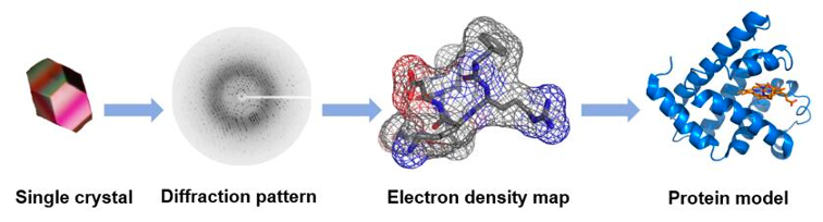
X-ray crystallography, also known as single-crystal X-ray diffraction, is a technique used to determine the atomic structure of molecules within crystalline forms. This process involves creating a crystal of the molecule of interest, which is then positioned on a goniometer and exposed to a focused beam of X-rays (Figure 2). The resulting diffraction pattern produced by the X-rays passing through the crystal allows for the determination of the atomic positions, chemical bonds, crystallographic disorder, and various other structural details. Interpreting the relationship between the diffraction pattern and the electron density requires complex mathematical calculations, specifically involving Fourier transforms, to generate a 3D model of the structure.
When collecting X-ray diffraction data from a crystal, we measure the intensities of diffracted waves scattered in all directions. These measurements give us the amplitudes but not the phase information needed to reconstruct an image (density map) of the molecule, which is known as the ‘phase problem’. This issue becomes more challenging with missing or poor data. In protein crystallography, phases are often obtained using atomic coordinates of a similar protein (molecular replacement, MR) or by identifying heavy atom positions. Heavy atoms scatter X-rays more strongly than lighter ones, helping us determine their positions within the crystal. By comparing diffraction patterns of the original crystal and one with added heavy atoms, we can deduce phase information through isomorphous replacement. Heavy atoms act as reference points to recover lost phase information, crucial for reconstructing the 3D structure of the molecule. Molecular replacement finds models that fit experimental intensities from known structures, typically needing to cover at least 50% of the total structure with a low Cα r.m.s.d. About 70% or more of PDB structures have been solved using this method, with the number rising as more homologous structures become available (Abergel 2013). Advances in de novo protein structure prediction have led to protocols like MR-Rosetta, QUARK, AWSEM-Suite, I-TASSER-MR, and Alphafold-guided MR, which generate native-like decoy structures useful for solving the phase problem (Wang, Gong, and Hendrickson 2025).
X-ray diffraction is a powerful technique that enables the acquisition of high-resolution atomic-level structures of both soluble and membrane proteins, whether as apoenzymes or holoenzymes bound to a substrate, cofactor, or drugs. However, the protein sample must be crystallizable (i.e., homogeneous), necessitating a substantial amount of very pure protein. A further limitation of X-ray structures is that they provide only one (or very few) static forms of the protein, and the locations of hydrogen atoms cannot be determined by conventional diffraction methods. Due to their single electron, hydrogen atoms are difficult to detect accurately with X-rays, which scatter at the electron density. Although hydrogen atoms can be predicted, this limitation still complicates some chemical analyses. Some proteins retain full functionality, permitting in crystallo experiments with certain enzymes (Chang, Zhou, and Gao 2023), but there are also numerous examples where crystallization may lead to a biased representation of the protein and result in structural artifacts.
2.2 Nuclear Magnetic Resonance
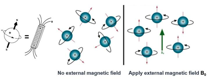
All atomic nuclei are charged, rapidly spinning particles that produce unique resonance frequencies for each atom. When a magnetic field is applied, an electromagnetic signal with a frequency characteristic of the magnetic field at the nucleus can be detected. This principle forms the basis of nuclear magnetic resonance (NMR, Figure 3).
It is important to note that the motion of the nucleus is not isolated; it interacts both intra- and intermolecularly with surrounding atoms. Consequently, nuclear magnetic resonance spectroscopy can provide structural information about specific molecules. For instance, in proteins, secondary structures such as α-helices, β-sheets, and turns indicate various arrangements of main chain atoms in three-dimensional space. The distances between atomic nuclei in these secondary structures, their interactions, and the dynamic properties of polypeptide segments all directly reveal the three-dimensional structure of proteins. These nuclear characteristics contribute to the spectroscopic behavior of the sample, yielding distinctive NMR signals. Computational interpretation of these signals facilitates the determination of the protein’s three-dimensional structure.
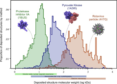
The primary advantage of the NMR method is that it allows for the direct measurement of the three-dimensional structure of macromolecules in their natural state in solution. NMR provides information about the dynamics and intermolecular interactions of these molecules. The resolution of the three-dimensional structure can extend to the subnanometer range. However, the NMR spectrum of large biomolecules is complex and challenging to interpret, limiting its application to analyzing large biomolecules, typically below 20-30 kDa (see Figure 4). Additionally, this technique requires relatively large amounts of pure samples (several milligrams) to achieve a reasonable signal-to-noise ratio.
2.3 Electron cryomicroscopy
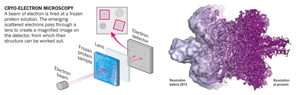
The fundamental principle of Cryo-EM is electron scattering, similar to other electron microscopy methods. Samples are prepared through cryopreservation prior to analysis. Then, an electron source is used as a light source to measure the sample. After the electron beam passes through the sample, a lens system converts the scattered signal into a magnified image recorded on the detector. A crucial subsequent step is signal processing, which transforms thousands of images of the particles in various orientations into a three-dimensional structure of the sample.
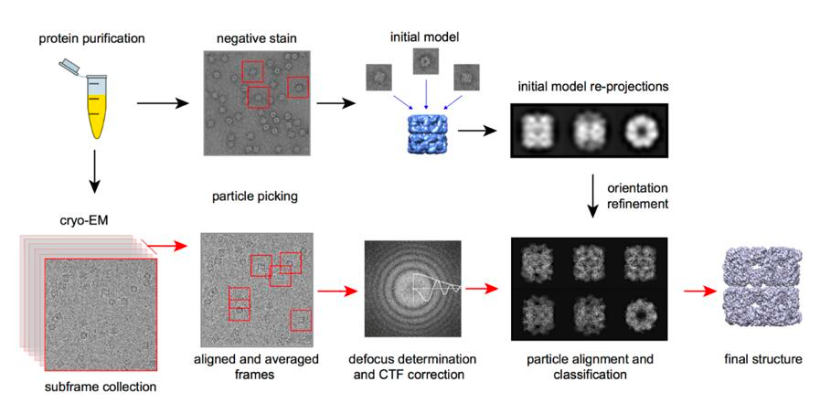
Traditionally, the use of electron microscopy methods for structural biology was limited to large macromolecular complexes, such as viral capsids (see Figure 4). Recently, it has also been applied to smaller particles. The number of protein structures determined by cryo-electron microscopy has significantly increased over the past 5-10 years (check it at PDB: https://www.rcsb.org/stats/all-released-structures). This increase is due to several technical improvements in the technique (Figure 6), including sample preparation and preservation, analysis, and processing, allowing for atomic-level imaging (Callaway 2020). These advancements were recognized by the awarding of the 2017 Nobel Prize in Chemistry to Jacques Dubochet, Joachim Frank, and Richard Henderson. .
CryoEM is commonly used today, especially for large molecular complexes or viral particles. It allows structures to be generated quickly, requires a minimal amount of protein, and can produce reliable data even with impurities present. However, new generation microscopes are typically only affordable for large institutions, and small particles often have a high level of noise. Additionally, processing a large number of images can be challenging when aiming to obtain high-quality structures.
3 Structural quality assurance
As mentioned at the outset of this section, every structure, regardless of its origin or method of determination, is susceptible to error. Experimentally determined structures are, in reality, models that have been constructed to align with experimental data. The quality of the initial data and the precision of the experimental procedures significantly influence the reliability of the structural outcomes. Similar to other scientific disciplines, independent experiments can yield related models of the same molecule, though there are typically variations; nonetheless, both models may still be considered accurate representations.
Check the detailed documentation about PDB validation report here.
3.1 Global parameters in experimentally-based structures
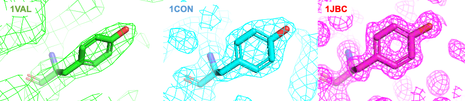
There are a number of different parameters that help us understand the quality and reliability of a structure. First, the resolution is a good indicator of the level of detail of the structure, as it can greatly affect affect how the experimental data are modeled.
Embedded reproduction of the Figure 7 with Mol*, which allow you to explore the structures.
Another important parameter is the R-factor, which is the difference between the structure factors calculated from the model and those obtained from the experimental data. That is, the R-factor is the deviation between the calculated diffraction pattern of the model and the original experimental diffraction pattern. Typically, good structures with a resolution of 1-3 Å, have an R-factor of 0.2 (i.e., 20% of deviation). However, it should be noted that this factor is usually reduced after iterative refinement, which downplays its use as an indicator of reliability. A more reliable factor is the Rfree factor. This is less susceptible to manipulation during refinement, as it is based on only a small portion of the experimental data (5-10%) that is not used during the refinement phase.
A more intuitive, but only qualitative, way to understand the precision of the coordinates of a given atom is the B-factor. The temperature value or B-factor correlates with the position errors, although its mathematical definition is more complex. Normal values for a B-factor are in the range of 14-30, while values above 30 usually indicate that the atom is in a flexible or disordered region, and atoms with a B-factor above 40 are often ruled out as too unreliable.
The root-mean-squared deviation (RMSD, see Structure alignment section) is a traditional estimator of the quality of NMR-solved structures. Regions with high RMSD values are those that are less defined by data. However, it should also be noted that this parameter can be also misleading, as it is highly dependent on the procedure used to generate and select the data that is submitted to the PDB. An experimentalist could reduce the RMSD by selecting the “best” few structures for deposition from a much larger draft. Note that the RMSD has many other applications, like comparing different structures or models from the same or related sequences.
In recent years, with the increase of quantity and quality of EM structures, new parameters have also been proposed. One of them, the Q-factor was recently introduced for validation of 3DEM/PDB structures. Briefly, the Q-factor score calculates the resolvability of atoms by measuring the similarity of the map values around each atom relative to a Gaussian-like function for a well resolved atom. A Q score of 1 means that the similarity is perfect, while a value close to 0 indicates low similarity. If the atom is not well placed in the map, a negative Q value can be given. Therefore, Q-factor values in the reports range from -1 to +1.
3.2 Stereochemical parameters
Since all structural models contain some degree of error and some of the global modeling parameters may be controversial, we can analyze the geometry, stereochemistry, and other structural properties of the model to evaluate structural models. These parameters compare a given structure to what is already known about that type of molecule based on our knowledge from high-resolution structures. This means that the structures in the current structure space define what is “normal” in a protein structure. The advantage of these analyses and derived parameters is that they do not take into account the process that leads to the model, only the final product and its reliability. The main disadvantage is that the current structure space is focused on proteins with known function and of biomedical or biotechnological interest.
One of the most common and powerful methods for assessing the stereochemistry of a protein is the Ramachandran plot, which was defined in 1963 and is still in use.
Another widely used analysis (available for all PDB structures) is the side chain torsion angles, usually measured as Side chain outliers. As described in the Introduction, the amino acid side chains also have some preferred conformations. Like the Ramachandran plot, the plot of the χ1-χ2 torsion angles can indicate problems with a protein model if the angle values are outside of the high density values.
Bad contact or clashes indicate a poor model. It is obvious that two atoms cannot be in the same (or a very close) location. We can define this as a situation where two unbound atoms have a center-to-center distance smaller than the sum of their van der Walls radii.
4 Protein structure display
4.1 Protein structure file formats
Experimental structural data from different methods are stored in different file formats. For instance, raw crystallographic data are usually stored as *.ccp4 files, but Cryo-EM or X-ray density maps can be stored in *.mrc or *.mtz files. Other complex file formats, such as the Extensible Markup Language *.xml, provide a framework for structure complex information and documents like protein structures.
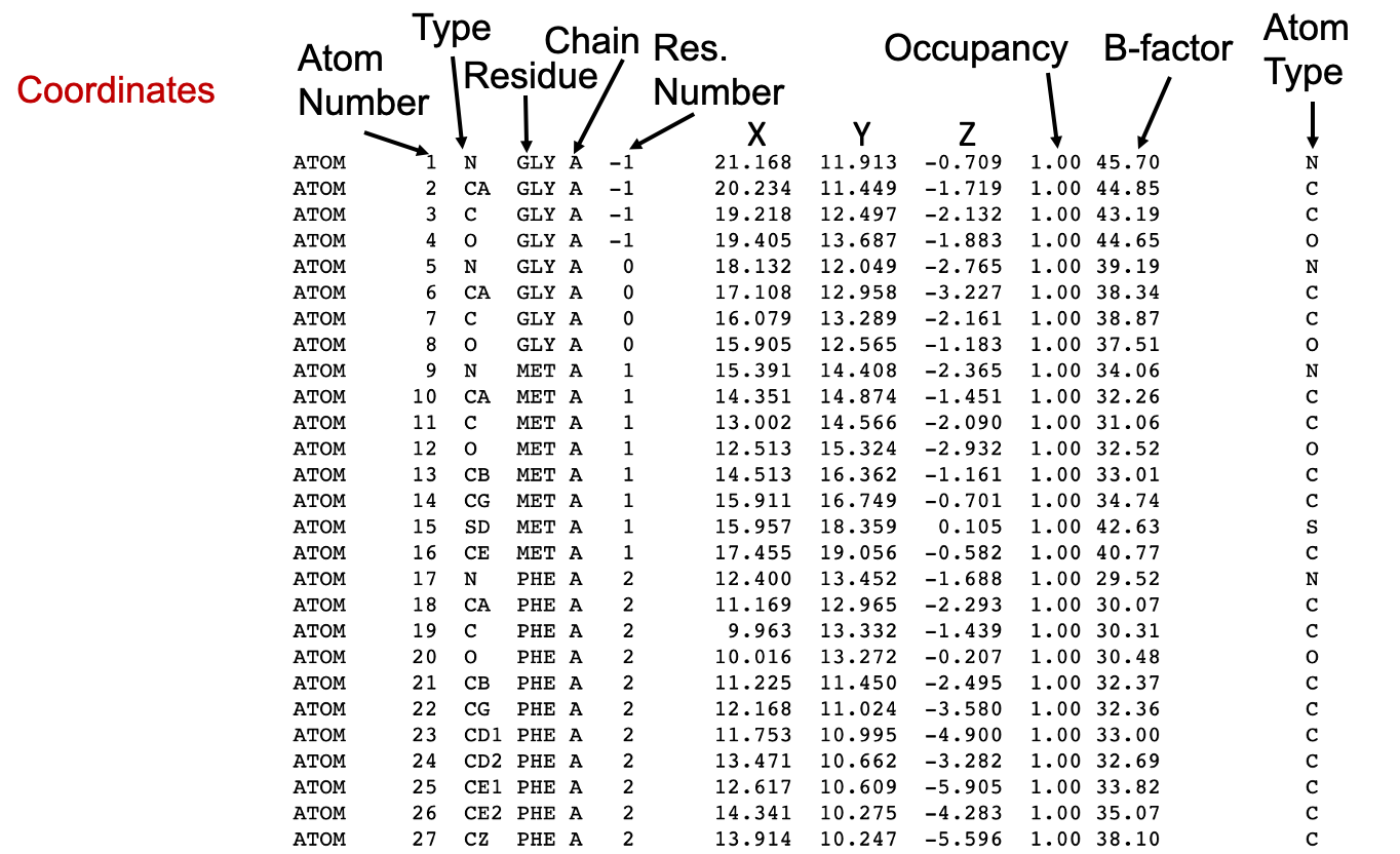
Along with the establishment of the Protein Data Bank, a simple and standardized format was developed. The Brookhaven or PDB format consists of line records in a fixed format describing atomic coordinates, chemical and biochemical features, experimental details of the structure determination, and some structural features such as secondary structure assignments, hydrogen bonding, or active sites. The current version is named PDBx/mmCIF) also incorporates the expanded crystallographic information file format (mmCIF), which allows the representation of large structures, complex chemistry, and new and hybrid experimental methods. Thus a *.pdb and *.cif files can be considered as identical files.
Check PDB-101 course about PDBx/mmCIF format at PDB RCSB site here.
Occupancy and B-factor
Except for the repetition of the atom type in the rightmost column, the last columns in the PDB file are the Occupancy and the temperature factor or the B-factor.
Macromolecular crystals consist of many individual molecules packed in a symmetrical arrangement. In some crystals there are slight differences between the individual molecules. For instance, a sidechain on the surface may wag back and forth between several conformations, or a substrate may bind in two orientations at an active site, or a metal ion may be detected as bound to only a few of the molecules. When researchers build the atomic model of these portions, they can use the occupancy to estimate the amount of each conformation observed in the crystal. Therefore, by definition, the sum of occupancy values for each atom must be 1. Usually, we see a single record for an atom, with an occupancy value of 1, indicating that the atom is found in all of the molecules in the same place in the crystal. However, if a metal ion binds to only half of the molecules in the crystal, the researcher sees a faint image of the ion in the electron density map and can assign an occupancy of 0.5 for this atom in the PDB structure file. For each atom, two (or more) atom records are included with occupancies such as 0.5 and 0.5, or 0.4 and 0.6, or other fractions of occupancies that sum to a total of 1.
On the other hand, the temperature value or B-factor is a measure of our confidence in the location of individual atoms, as described above (Section 3). If you find an atom with a high temperature factor on the surface of a protein, keep in mind that this atom is likely to be moving around a lot and that the coordinates given in the PDB file are only a possible snapshot of its location. Thus, an atom dataset with an occupancy < 1 may have a low B-factor if that position is safe.
As you can imagine, this column is also used by computationally derived models to indicate a confidence value that can be parsed for diverse purposes, including structure coloring.
4.2 Biological macromolecules display applications
PyMOL
PyMOL is a very powerful molecular visualization system written originally by Warren DeLano. It was released in 2000 and soon became very popular. It’s currently commercialized under License by Schrödinger but a free license for teaching can be requested. Also, open source code is available on GitHub that can be installed on Linux or MAC. More info on Wikipedia. You can also check this quick Reference guide
PyMOL allows working with different structures representation, but also with raw experimental data in different formats.
PyMOL is written in Python and can be used with interactive menus and also with command line. There are a lot of resources that can help you with PyMOL, like a Documentation Reference Wiki or a community-supported PyMOLWiki. Moreover, it allows the implementation of new functionalities as plugins (Rosignoli and Paiardini 2022), like PyMod or DockingPie, among others. PyMod (Janson and Paiardini 2021) is designed to act as simple and intuitive interface between PyMOL and several bioinformatics tools (i.e., PSI-BLAST, Clustal Omega, HMMER, MUSCLE, CAMPO, PSIPRED, and MODELLER). Starting from the amino acid sequence of the target protein, PyMod is designed to carry out the main steps of the homology modeling process (that is, template searching, target-template sequence alignment and model building) in order to build a 3D atomic model of a target protein (or protein complex). The integration with PyMOL facilitates a detailed analysis of the modeling process.
You can write Pymol scripts just by listing commands in a file, one command per line, appearing as they would be entered at the PyMOL command prompt. The standard extension for a PyMOL script is .pml.
Moreover, you can write more complex Python-based scripts, as detailed in the wiki
Finally, as any Python-based program, it can be used within Jupyter notebooks (see https://www.computer.org/csdl/magazine/cs/2021/02/09354947/1rgCkrAJCko).
UCSF ChimeraX
ChimeraX (Pettersen et al. 2021) is a fully open source software, developed by the UCSF as a renovated version of the former Chimera software, with versions for Linux, MacOS, and Windows. It aims to be a comprehensive structural biology tool, but it is more widely known for its capacities for EM maps. As any other open source software, it has gained new and exciting capacities in the last years, like Virtual Reality capabilities or Alphafold2 modeling.
There is an excellent ChimeraX User Guide, with examples at the RBVI@UCSF site here.
Molecular structures on your website: Mol* and others
LiteMol Viewer is a powerful HTML5 web application for 3D visualization of molecules and other related data. It is used in a web browser, eliminating the need for external software and also allowing the integration with third-party sites as an embedded plugin. More information about LiteMol can be found on Sehnal et al. (2017), the wiki, or YouTube tutorials.
The same philosophy applies to other open-source viewers that were developed later and are now more widely used, like NGL Viewer and Mol* Sehnal et al. (2021), used in RCSB-PDB and PDBe sites for 3D visualization of structures. With Mol* you can save your work session in molj (without the actual structures) or molx (with embedded structures) formats, as in the Figure 8 above.
Finally, for computational scientists, there are also many libraries that allow 3D molecules representation, like 3Dmol Javascript library and its Python wrapper Py3Dmol, which you can use in Colab, Jupyter, Quarto or any other Python notebook (see code examples here or here).
4.3 Parsing multiple structures
As PDB files are text files, you can easily write your own scripts to parse structures and process their data. Moreover, Python and R offer several robust libraries for parsing and visualizing protein structures. Biopython is widely utilized for parsing PDB files, while libraries such as NGL, Py3Dmol, or matplotlib (with creative geometry) are effective for visualization. Biopython is essential for parsing and working with protein structure data, irrespective of the chosen visualization library.
Py3Dmol: Suitable for basic visualizations and web embedding.
NGL: Highly powerful and feature-rich, offering interactive capabilities, commonly used in bioinformatics. Requires Jupyter extensions.
ProDy: Protein structure analysis and dynamics as well as insights that make protein visualizations more informative. It’s not a standalone visualization library but a valuable companion to libraries like NGL, Py3Dmol, and Matplotlib.
- py3DMol: https://colab.research.google.com/github/CCBatIIT/modelingworkshop/blob/main/labs/1-1/py3DMol.ipynb
- py3DMol and MDAnalysis: https://colab.research.google.com/github/pb3lab/ibm3202/blob/master/tutorials/lab02_molviz.ipynb
- py3DMol and NGLView: https://colab.research.google.com/github/pb3lab/ibm3202/blob/master/tutorials/lab02_molviz.ipynb
In R, there are also packages designed for working with protein structures. The bio3d package is fundamental in R for bioinformatics, providing functions for reading PDB files, analyzing protein structures, and generating basic visualizations. It can perform calculations such as distances, RMSDs, and other structural analyses. There is also a very useful Mol* Quarto extension, which I used on this site. Mol* can be very easily integrated in many third party services and in your own website.
Other applications that you may know, hear about or came into but are now discontinued are:
SwissPDBViewer (aka DeepView), developed to work with SWISS-MODEL homology modeling app, is an application that provides a user-friendly interface allowing to analyze several proteins at the same time. It has currently fallen in disuse as the last version (4.1) is only a 32 bits application.
RasMol and OpenRasMol were developed initially in 1992 and its last release was in 2009. It was a pioneer as a simple molecular display open-source application, but it is outdated nowadays.