Advanced homology modeling
1 From homology modeling to threading
Although we do not intend to describe in detail the evolution of modeling methods, I briefly outline below the origin and transformation of advanced protocols that outperform the classical single-template homology modeling during the last three decades. This step-wise evolution of modeling methods is the origin of the revolution of Alphafold and related protocols, which we will discuss in the next section.
Threading or Fold-recognition methods
As mentioned earlier, the introduction of HMM-based profiles during the first decade of this century led to a great improvement in template detection and protein modeling in the twilight zone, i.e., proteins with only distant homologs (<25-30% identity) in databases. In order to exploit the power of HMM searches, those methods naturally evolved into iterative threading methods, based on multitemplate model construction, implemented in I-TASSER (Roy, Kucukural, and Zhang 2010), Phyre2 (L. A. Kelley et al. 2015), and RosettaCM (Song et al. 2013), among others. These methods are usually referred to as Threading or Fold-recognition methods. Note that the classification of modeling methods is often blurry. The current version of SwissModel and the use of HHPred+Modeller already rely on HMM profiles for template identification and alignment; being thus strictly also fold-recognition methods.
Both terms can be often used interchangeably, although some authors see Fold-Recognition as any technique that uses structural information in addition to sequence information to identify remote homologies, while Threading would refer to a more complex process of modeling including remote homologies and also the modeling of pairwise amino acid interactions in the structure. Therefore, HHPRED is a fold-recognition method and its use along with Modeller, could be indeed considered threading.
The Iterative Threading ASSembly Refinement (I-TASSER) from Yang Zhang lab is one of the most widely used threading methods and servers. This method was was ranked as the No 1 server for protein structure prediction in the community-wide CASP7, CASP8, CASP9, CASP10, CASP11, CASP12, CASP13, and CASP14 experiments. I-TASSER first generates three-dimensional (3D) atomic models from multiple threading alignments and iterative structural assembly simulations that are iteratively selected and improved. The quality of the template alignments (and therefore the difficulty of modeling the targets) is judged based on the statistical significance of the best threading alignment, i.e., the Z-score, which is defined as the energy score in standard deviation units relative to the statistical mean of all alignments.
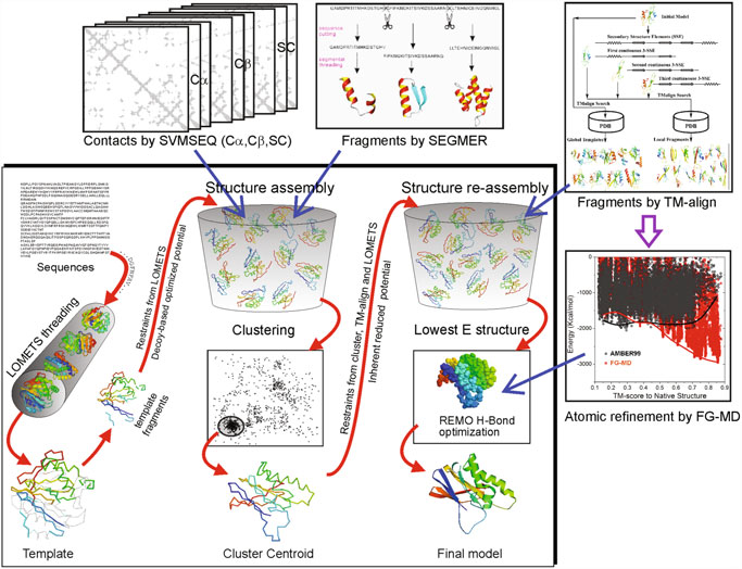
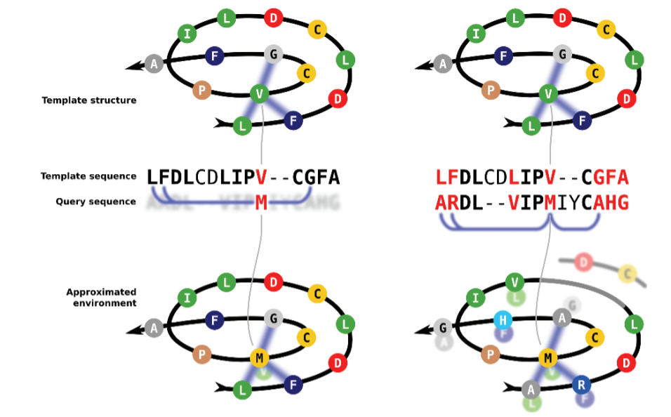
First, I-TASSER uses Psi-BLAST against curated databases to select sequence homologs and generate a sequence profile. That profile is used to predict the secondary structure and generate multiple fragmented models using several programs. The top template hits from each threading program are then selected for the following steps. In the second stage, continuous fragments in threading alignments are excised from the template structures and are used to assemble structural conformations of the sections that aligned well, with the unaligned regions (mainly loops/tails) built by ab initio modeling. The fragment assembly is performed using a modified replica-exchange Monte Carlo random simulation technique, which implements several replica simulations in parallel using different conditions that are periodically exchanged. Those simulations consider multiple parameters, including model statistics (stereochemical outliers, H-bond, hydrophobicity…), spatial restraints and amino acid pairwise contact predictions (see below). In each step, output models are clustered to select the representative ones for the next stage. A final refinement step includes rotamers modeling and filtering out steric clashes.
One interesting thing about I-TASSER is that it is integrated within a server with many other applications, including some of the tools that I-TASSER uses and other advanced methods based on I-TASSER, like I-TASSER-MTD for large, multidomain proteins or C-I-TASSER that implements a deep learning step, similar to Alphafold2 (see next section).

RosettaCM is an advanced homology modeling or threading algorithm by the Baker lab, implemented in Rosetta software and the Robetta webserver. RossetaCM provides accurate models by breaking up the sequence into fragments that are aligned to a set of selected templates, generating accurate models by a threading processes that uses different fragments from each of the templates. Additionally it uses minor ab initio folding to fill the residues that could not be assigned during the threading. Then, the model is closed by iterative optimization steps that include Monte Carlo sampling. Finally, an all-atom refinement towards a minimum of free energy (Song et al. 2013).
De novo or ab initio modeling used to mean modeling a protein without using a template. However, this strict definition is blurred in the 2000s (decade) by advanced methods that use fragments. Threading protocols such as RosettaCM and I-Tasser, among others, use fragments that may or may not come from homologous protein structures or not. Therefore, they cannot be classified as homology modeling, but they are sometimes referred to as comparative or hybrid methods.
Scoring functions in threading and deep-learning protein modeling
In protein modeling, various scoring functions are used to evaluate the similarity of protein structures. As you know, the Root-Mean-Square Deviation (RMSD) measures three-dimensional similarity by calculating the RMSD of the Cα atomic coordinates after structural alignment. However, it is sensitive to outliers and may overlook good models. TM-Score is a normalized alternative to RMSD, ranging from 0 to 1, which considers the length of the protein and is less influenced by outliers.
In CASP, the score of the models is based on the Global Distance Test (GDT), often expressed as a percentage between 0 and 100, which measures the number of residues within a set distance cutoff. Specifically, the GDT-TS calculates the average GDT for 1, 2, 4, and 8 Å cutoffs. Similar to RMSD, the GDT score is length-dependent, as its average score for random structure pairs follows a power-law dependence on protein size. To address this, the GDT-TS Z-score, used in RosettaCM, indicates data quality and dispersion based on mean and standard deviation values. This use of the Z-score or standard scores is common in mathematics, reflecting how many standard deviations a raw score is from the mean.
Finally, the plDDT, or per-residue estimate lDDT (Mariani et al. 2013) used in AlphaFold and related methods, provides a per-residue normalized score of Cα-atomic superposition-free distance, with values ranging from 0 to 100. This scoring can refer to either a single structure or an ensemble, offering detailed insights into protein modeling accuracy. Additionally, if a protein region is naturally highly flexible or intrinsically disordered, in which case it does not have any well-defined structure, will also have a lower lDDT (Wilson, Choy, and Karttunen 2022).
2 From contact maps to pairwise high-res feature maps
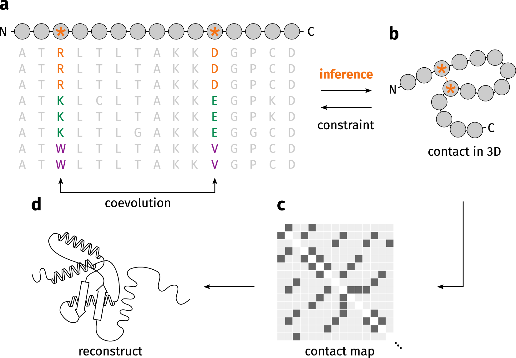
As introduced earlier, a contact map represent the pairwise distances between all amino acid residues in a three‑dimensional protein structure using a binary two‑dimensional matrix.
More than thirty years ago, it was already suggested that reliable residue–residue contact information could, on its own, determine a protein’s fold (Olmea and Valencia 1997). However, incorporating contact maps into protein modeling proved difficult, as accurately predicting these contacts remained a major challenge. The emergence of direct‑coupling analysis (DCA), which infers residue coevolution from multiple sequence alignments (MSAs) as illustrated in Figure 4, greatly improved the quality of contact predictions. This advance enabled their use in protein folding approaches such as PSICOV (Jones et al. 2012) and Gremlin (Kamisetty, Ovchinnikov, and Baker 2013). Even so, when proteins lack sufficient sequence homologs, the resulting contact predictions are often of limited reliability, making precise contact‑guided protein modeling still problematic.
Implementation of several layers of information processed by neural network and deep learning methods
Deep learning is a sub-field of machine learning based on artificial neural networks (NNs). Neural networks were initially introduced in the late 1940s and 1950s but gained prominence again in the 2000s with the rise of computational capacities and the use of GPUs. Essentially, an NN uses multiple interconnected layers to transform various inputs, such as MSAs and high-resolution contact maps, into complex features that can then predict intricate outputs like a 3D protein structure. NNs aim to simulate the behavior of the human brain, processing large amounts of data and learning from it. Deep learning utilizes multiple-layer NNs to optimize and refine accuracy.
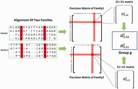
The next complexity level in contact maps involves applying them to distantly related proteins by comparing sets of DCA from different protein families, sometimes referred to as joint evolutionary coupling analysis (Figure 5). This method requires processing massive amounts of information, which increases computational demands. Hence, the use of trained neural networks and advanced deep-learning methods has significantly enhanced protein modeling capabilities.
In this context, the introduction of supervised machine learning methods that predict contacts has outperformed DCA methods by employing multilayer neural networks (Jones et al. 2015; Ma et al. 2015; Wang et al. 2017; Yang et al. 2020). These methods incorporate high-resolution contact maps (Figure 6), containing enriched information that includes not only contacts but also distances and angles, represented in a heatmap-like probability scale.
