Protein Structures
1 Obtaining and working with protein structures

The surrealist Belgian painter René Magritte created a collection of surrealistic paintings entitled La trahison des images (1928–1929). The most renowned of those paintings show a smoking pipe and the following caption underneath: “Ceci n’est pas une pipe” (This is not a pipe). Yes, indeed! It is actually the painting of a pipe.
Similarly, a picture of a protein, or a PDB file with the coordinates of a protein structure, is not a protein. It is a representation of ONE possible structure of that protein. Even experimentally determined structures have two main limitations that we should always keep in mind: (1) they are a fixed structure (except RMN-based) whereas proteins in vivo are flexible and dynamic and (2) they are subjected to experimental error and they often contain regions of low reliability (see below Section 3). Moreover, even experimentally obtained macromolecular structures are to some degree models, with a variable ratio between experimental data and computational prediction to match the experimental data (X-ray diffraction, cryo-EM density maps, NMR, SAXS, FRET…) with previously known structures or prediction models. Obviously, that does not mean that protein structures are useless, they can be very useful, but we must be aware of the limitations as well as the applications.
2 Experimental determination of protein structures
The structure helps to understand the molecular mechanism of protein function at a higher level of detail. The 3D representation can help to orientate different domains/motifs/residues of interest. This can be essential to understand the analysis of population or pathogenic variants, drug design, and protein engineering. Moreover, the structures can also help to predict protein function and evolution, as they are more conserved than sequence, i.e., the protein structure space is smaller than the sequence space. However, obtaining detailed and reliable structural data can be technically difficult and time-consuming and, as we will see, modeling protein structures can be often a good complement or alternative. Experimentally-obtained structures usually rely on three alternative techniques, X-ray crystallography, nuclear magnetic resonance (RMN), or electron cryomicroscopy (CryoEM).
2.1 X-Ray crystallography or single crystal X-ray diffraction
The X-Ray crystallography or single crystal X-ray diffraction is a method to determine the atomic structure of molecules in regular, crystalline structures. It requires the generation of a crystal of the molecule of interest that is then mounted on a goniometer and illuminated or irradiated with a focused beam of X-rays. The diffraction pattern of the X-rays at the other side of the crystal allow the determination of the atoms positions, as well as their chemical bonds, their crystallographic disorder, and various other information. However, the link between the diffraction pattern and the electron density is not trivial and requires some complex maths, called Fourier transforms.
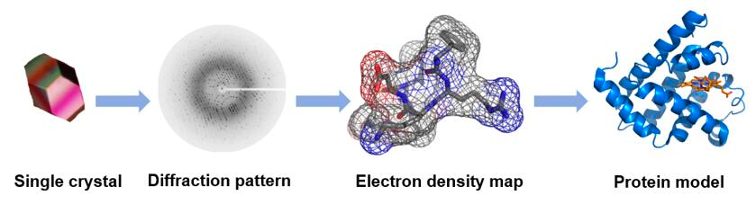
X-ray is a powerful method that allows obtaining high-resolution structures at the atomic level of soluble or membrane proteins, either as an apoenzyme or as a holoenzyme bound to substrate, cofactor or drugs. However, the sample must be crystallizable (i.e. homogeneous), which requires quite an amount of very pure protein. Another con of X-ray structures is that, as mentioned, you only obtain one (or very few) static forms of the protein and the location of hydrogen atoms cannot be determined by conventional diffraction methods—the fact that they have only one electron—makes them very hard to detect with x-rays accurately because x-rays scatter from the electron density. They can be predicted, but that still hinders some chemical analysis.
2.2 Nuclear Magnetic Resonance
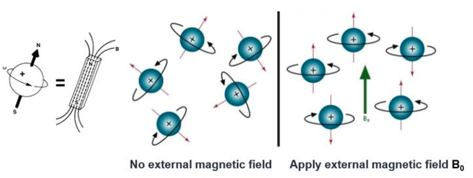
All atomic nuclei are charged, fast spinning particles, which gave rise to resonance frequencies that are different for each atom. Therefore, if we apply a magnetic field we can obtain an electromagnetic signal with a frequency characteristic of the magnetic field at the nucleus. That is the basis of nuclear magnetic resonance (NMR).
Also, we should consider that the movement of the nucleus is not isolated–it interacts with the surrounding atoms both intra- and inter-molecularly. Thus, through nuclear magnetic resonance spectroscopy, structural information of a given molecule can be obtained. Taking protein as an example, its secondary structure, such as α-helix, β-sheet, turn, circular, and curl, reflect the different arrangement of the main chain atoms of protein molecules three-dimensionally. The spacing of the atomic nuclei in different secondary domains, the interaction between nuclei, and the dynamic characteristics of polypeptide segments all directly reflect the three-dimensional structure of proteins. These nuclear features all contribute to spectroscopic behaviors of the analyzed sample, thus providing characteristic NMR signals. Interpretation of these signals by computer-aided methods leads to deciphering of the three-dimensional structure.
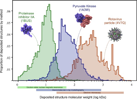
The most important feature of the NMR method is that the three-dimensional structure of macromolecules in the natural state can be measured directly in solution, and NMR may provide unique information about dynamics and intermolecular interactions. The resolution of the macromolecular three-dimensional structure can be as low as sub nanometer. However, the NMR spectrum of biomolecules with large molecular weight is very complicated and difficult to interpret, thereby limiting the application of NMR in analyzing large biomolecules, often below 20-30 kDa (see Figure 4). Additionally, this technique requires relatively large amounts of pure samples (on the order of several mg) to achieve a reasonable signal to noise level.
2.3 Electron cryomicroscopy
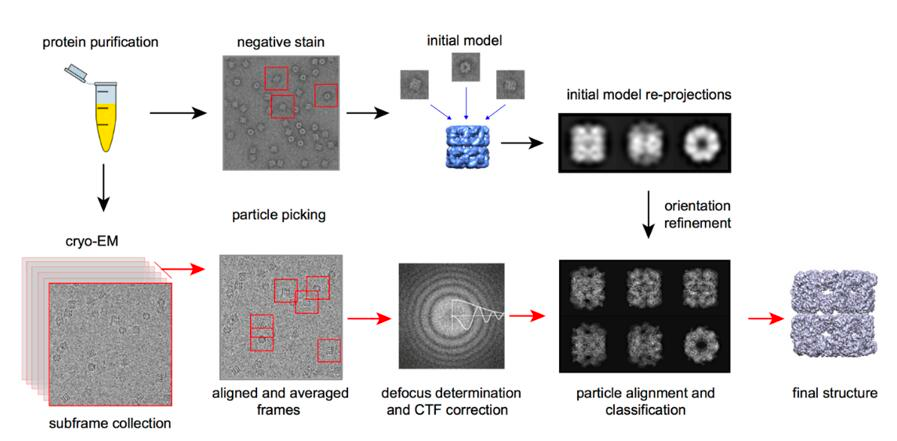
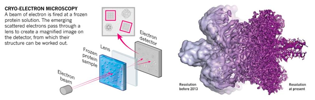
The essential mechanism of Cryo-EM is the same of any electron microscopy method, i. e., electron scattering. Samples are prepared through cryopreservation prior to analysis. The coherent electrons are used as a light source to measure the sample. After the electron beam passes through the sample, a complex lens system converts the scattered signal into a magnified image recorded on the detector. A key subsequent step is signal processing, that transform thousands of images of the particles in any orientation into a three-dimensional structure of the sample.
The use of electron microscopy methods for structural biology was traditionally limited to very large macromolecular complexes, like viral capsids, and only recently it could be used for smaller particles (see Figure 4). The number of protein structures being determined by cryo-electron microscopy is growing at an explosive rate in the last 5-10 years. This is thanks to several technical improvements in the technique, spanning sample preparation, analysis and processing that allow obtaining pictures at the atomic level (Callaway 2020). This advances were acknowledged by the 2017 Nobel Prize in Chemistry to Jacques Dubochet, Joachim Frank and Richard Henderson.
CryoEM is widely use nowadays because, particularly for large molecular complexes or viral particles. Structures can be generated quickly, as it does not require a high amount of protein and it can generate good data even in the presence of impurities. However, new generation microscopes are only affordable by large institutions and small particles can have a high level of noise. Moreover, processing a large amount of images can be limiting to obtain high-quality structures.
3 Structural quality assurance
As outlined at the beginning of this section, regardless of the origin or determination method, any structure is subjected to error. Experimentally-based structures are actually models that match with the data. The quality of the original data and the care with which the experiments have been performed will determine the reliability of the structural results. As in any other scientific discipline, independently performed experiments can arrive to related models of the same molecule but almost always there are differences; however both can be good models.
Check the detailed documentation about PDB validation report here.
3.1 Global parameters in experimentally-based structures
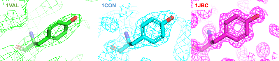
There are a number of diverse parameters that help us to understand the quality and reliability of an structure. First, the resolution is a good indicator of the level of detail of the structure, as it can strongly affect affect how the experimental data is modeled.
Other important parameter is the R-factor, which assess the difference between the structure factors calculated from the model and those obtained from the experimental data. This is, the R-factor is the deviation of the calculated diffraction pattern of the model and the original experimental diffraction pattern. Typically, good structures with a resolution around 1-3 Å, will have an R-factor of 0.2 (i.e., 20% of deviation). However, it should be noted that this factor is usually reduced after iterative refinement, which downplays its use as an indicative of reliability. A more reliable factor is the Rfree. This is less susceptible to manipulation during refinement, as it is based only in a small fraction of the experimental data (5-10%) that is not used throughout the refinement stage.
A more intuitive, but only qualitative, way of understand the presicion of a given atom’s coordinates is the B-factor. The temperature value or B-factor correlates with the positional errors, although its mathematical definition is more complex. Normal values for a B-factor are within the range 14-30, whereas values above 30 usually indicate that the atom is within a flexible or disordered region, and atoms with a B-factor over 40 are often excluded as being too unreliable.
The root-mean-squared deviation (RMSD, see Structure alignment section) is a traditional estimator of the quality of NMR-solved structures. Regions with high RMSD values are those that are less defined by data. However, it should be also noted that this parameter can be also misleading as it is highly dependent on the procedure used to generate the and selection the data that is submitted to the PDB. An experimentalist could reduce the RMSD by choosing the “best” few structures for deposition from a much larger draft. Note that the RMSD has many other applications, like comparing different structures or models from the same or related sequences.
In the last years, along with the boost in quantity and quality of EM structures, new parameters have been proposed. One of them, the Q-factor has been recently implemented for validation of 3DEM/PDB structures. Briefly, the Q-score calculates the resolvability of atoms by measuring similarity of the map values around each atom relative to a Gaussian-like function for a well resolved atom. Q-score of 1 indicates that the similarity is perfect whilst closer to 0 indicates the similarity is low. If the atom is not well placed in the map then a negative Q-score value may be reported. Therefore, Q-score values in the reports will be in a range of -1 to +1.
3.2 Stereochemical parameters
Given that all structural models contain some degree of error and some of the modeling global parameters can be controversial, we can analyze the model’s geometry, stereochemistry, and other structural properties to assess structural models (experimentally or computationally obtained). These parameters compare a given structure (protein or nucleic acid) against what is already known about this kind of molecule, based on our knowledge from high-res structures. That means that the (best) structures in the current structural space define what is “normal” in a protein structure. The advantage of these analyses and derived parameters is that they do not consider the process that leads to the model, they only consider the final product and its reliability. The main disadvantage is that the current structural space is biased to proteins of known function and with biomedical or biotechnological interest.
One of the most common and powerful methods to asses the stereochemistry of a protein is the Ramachandran plot, defined in 1963 and still in use.
Another widely used analysis (and available for all PDB structures) is the side chain torsion angles, usually measured as Side chain outliers. As outlined in the Introduction, amino acid side chains also have some preferred conformations. Like the Ramachandran plot, a plot of the χ1-χ2 torsion angles can indicate problems with a protein model when angle values are outside of the high density values.
Bad contact or clashes indicate a bad model. It is obvious that two atoms cannot be in the same (or very close) spot. We can define this as a situation where two nonbonded atoms have a center-to-center distance that is smaller than the sum of their van der Walls radii.
4 Protein structure display
4.1 Protein structure file formats
Experimental structural data from different methods is stored in different file formats. For instance, crystallographic raw data is usually saved as *.ccp4 files, but Cryo-EM or X-ray density maps can be stored in *.mrc or *.mtz files. Other complex file formats, such as the Extensible Markup Language *.xml, provide a framework for structure complex information and documents like protein structures.
Along with the establishment of the PDB, a simple format was developed. The PDB format consist of a collection of fixed format records that describe the atomic coordinates, chemical and biochemical features, experimental details of the structure determination, and some structural features such as secondary structure assignments, hydrogen bonding, or active sites. The current version is named PDBx/mmCIF)also incorporates the expanded crystallographic information file format (mmCIF), allowing the representation of large structures, complex chemistry, and new and hybrid experimental methods. Thus a *.pdb and *.cif files can be considered as identical files.
Check PDB-101 course about PDBx/mmCIF format here.
4.1.1 Occupancy and B-factor
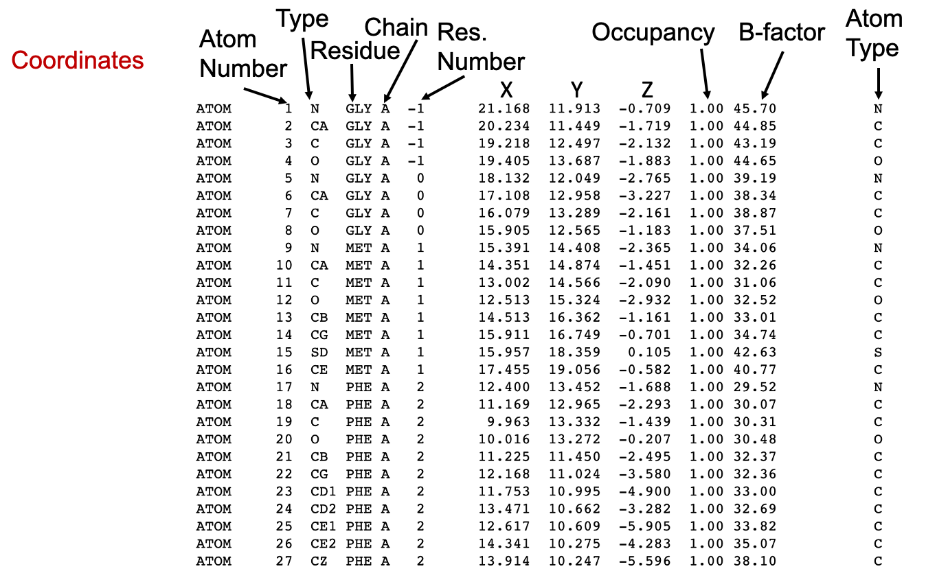
Disregarding the repetition of atom type in the rightmost column, the last columns in the PDB file are the Occupancy and the temperature factor or the B-factor.
Macromolecular crystals are composed of many individual molecules packed into a symmetrical arrangement. In some crystals, there are slight differences between each of these molecules. For instance, a sidechain on the surface may wag back and forth between several conformations, or a substrate may bind in two orientations in an active site, or a metal ion may be bound to only a few of the molecules. When researchers build the atomic model of these portions, they can use the occupancy to estimate the amount of each conformation that is observed in the crystal.
Thus, by definition, the sum of occupancy values for each atom must be 1. Usually, we will see a single record for an atom, with an occupancy value of 1, indicating that the atom is found in all of the molecules in the same place in the crystal. However, if a metal ion binds to only half of the molecules in the crystal, the researcher will see a weak image of the ion in the electron density map, and can assign an occupancy of 0.5 in the PDB structure file for this atom. Two (or more) atom records are included for each atom, with occupancies like 0.5 and 0.5, or 0.4 and 0.6, or other fractional occupancies that sum to a total of 1.
On the other hand, temperature value or B-factor is a measure of our confidence in the location of each atom, as discussed above (Section 3). If you find an atom on the surface of a protein with a high temperature factor, keep in mind that this atom is probably moving a lot, and that the coordinates specified in the PDB file are only one possible snapshot of its location. Thus, an atom record with an occupancy <1 can have a low B-factor if that position is certain.
As you can imagine, this column is also used by computationally-derived models to include a confidence value.
4.2 Biological macromolecules display applications
4.2.1 PyMOL
PyMOL is a very powerful molecular visualization system written originally by Warren DeLano. It was released in 2000 and soon became very popular. It’s currently commercialized under License by Schrödinger but a free license for teaching can be requested. Also, open source code is available on GitHub that can be installed on Linux or MAC. More info on Wikipedia. You can also check this quick Reference guide
PyMOL allows working with different structures representation, but also with raw experimental data in different formats.
PyMOL is written in Python and can be used with interactive menus and also with command line. There are a lot of resources that can help you with PyMOL, like a Documentation Reference Wiki or a community-supported PyMOLWiki. Moreover, it allows the implementation of new functionalities as plugins, like PyMod or DockingPie, among others. PyMod (Janson and Paiardini 2021) is designed to act as simple and intuitive interface between PyMOL and several bioinformatics tools (i.e., PSI-BLAST, Clustal Omega, HMMER, MUSCLE, CAMPO, PSIPRED, and MODELLER). Starting from the amino acid sequence of the target protein, PyMod is designed to carry out the main steps of the homology modeling process (that is, template searching, target-template sequence alignment and model building) in order to build a 3D atomic model of a target protein (or protein complex). The integration with PyMOL facilitates a detailed analysis of the modeling process.
Finally, as any Python-based program, it can be used within Jupyter notebooks (see https://www.computer.org/csdl/magazine/cs/2021/02/09354947/1rgCkrAJCko).
4.2.2 UCSF ChimeraX
ChimeraX (Pettersen et al. 2021) is a fully open source software, developed by the UCSF as a renovated version of the former Chimera software, with versions for Linux, MacOS, and Windows. It aims to be a comprehensive structural biology tool, but it is more widely known for its capacities for EM maps. As any other open source software, it has gained new and exciting capacities in the last years, like Virtual Reality capabilities or Alphafold2 modeling.
4.2.3 LiteMol and others
LiteMol Viewer is a powerful HTML5 web application for 3D visualization of molecules and other related data. It is used in a web browser, eliminating the need for external software and also allowing the integration with third-party sites as an embedded plugin, as it is in the PDBe site. More information about LiteMol can be found on Sehnal et al. (2017), the wiki, or YouTube tutorials.
The same phylosopy applies to other open-source viewers like NGL Viewer and Mol*. However, since LiteMol was developed by the EMBL-EBI and it is used in ePDB site, it has become more popular.
Other applications that you may know or came into are:
SwissPDBViewer (aka DeepView), developed to work with SWISS-MODEL homology modeling app, is an application that provides a user-friendly interface allowing to analyze several proteins at the same time. It has currently fallen in disuse as the last version (4.1) is only a 32 bits application.
RasMol and OpenRasMol were developed initially in 1992 and its last release was in 2009. It was a pioneer as a simple molecular display open-source application, but it is outdated nowadays.
5 PyMOL Practice
Our PyMOL Practice has two parts.
5.1 PART A: A 10-steps self-guided practice
This is a Evernote note that you can consult online and also copy into your Evenote account if you wish.
5.2 PART B: PyMOL Challenge
Make a ready-to-publish picture of your favorite protein. As a suggestion, you can reproduce the top panels in the Figure 1B of Gao et al. (2020), but any structure involving more than one domain and/or with a substrate/cofactor molecule can be a good challenge.