Homology Modeling

1 Modeling protein structures: Mind the gap

The number of protein sequences in databases growth exponentially during the last decades, particularly after the revolution of high throughput sequencing methods.

Figure 1: Number of entries in UniProt/TrEMBL (release 2022_2).

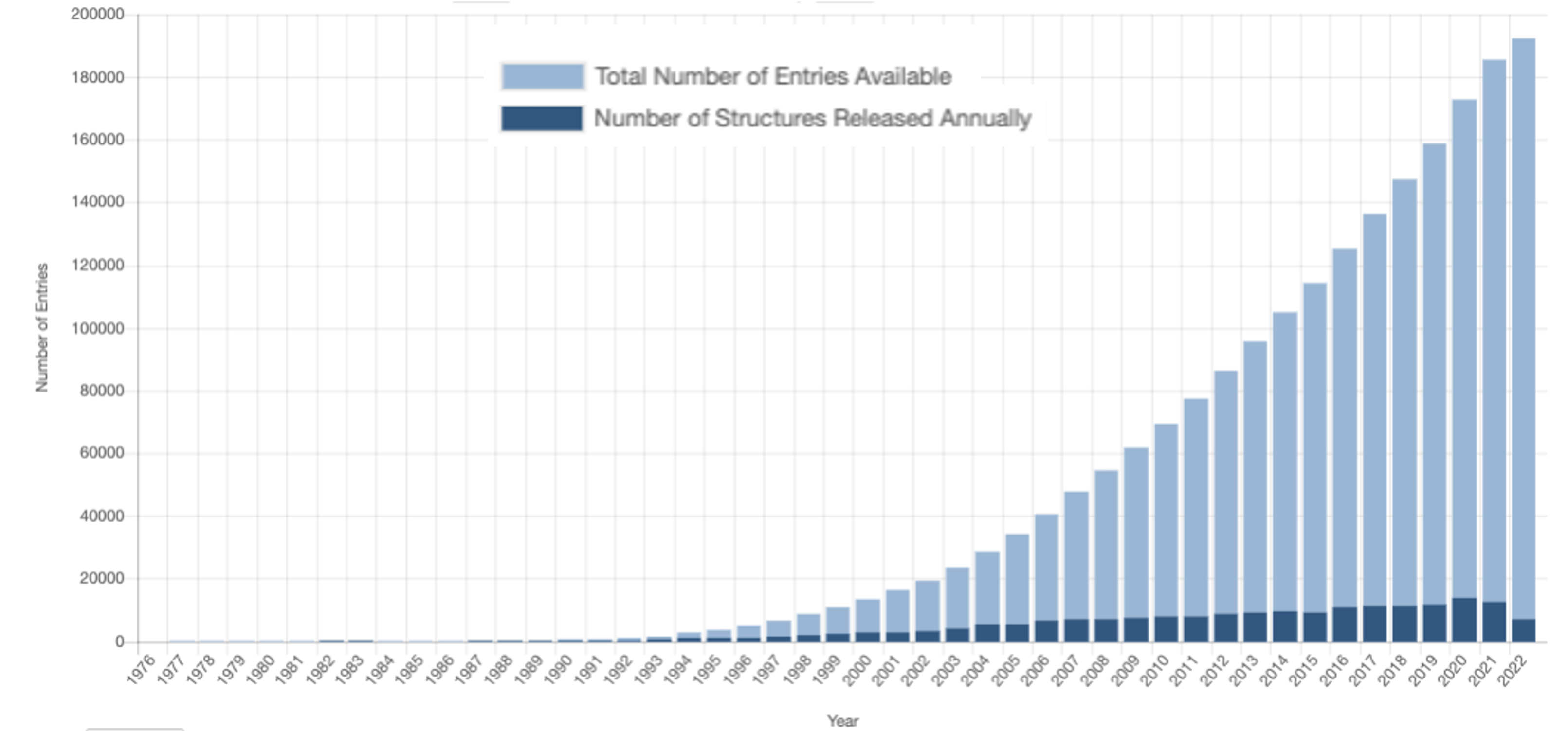
However, experimental determination of 3D protein structures is often difficult, time-consuming, and subjected to limitations, such as experimental error, data interpretation and modeling new data on previously released structures. Thus, despite substantial efforts that started at the beginning of the 21st century to implement high-throughput structural biology methods (see for instance Manjasetty et al. 2008), the availability of protein structures is more than 1,000 times less than the number of sequences (>226M sequences for Uniprot and ∽195k structures in RCSB Protein Databank in August 2022). This difference is called the protein structure gap and it is constantly widening (Muhammed and Aki-Yalcin 2019).

Figure 2: Number of macromolecular structures in RCSB PDB database (accessed 6th July 2022).

Thus, an accurate prediction of the 3D structure of any given protein is needed to make up for the lack of experimental data.

1.1 Are protein structures predictable at all?

Amino acid properties determine the phi and psi angles that eventually shape the higher structural levels. Protein folding might be more complex though, as it should be coupled to protein synthesis.

One can think that complexity and diversity of protein structures in the nature may be huge. Indeed, upon their determination of the three-dimensional globular structure (myoglobin, 1958), John Kendrew and his coworkers seemed very disappointed (Kendrew et al. 1958):

Perhaps the most remarkable features of the molecule are its complexity and its lack of symmetry. The arrangement seems to be almost totally lacking in the kind of regularities which one instinctively anticipates, and it is more complicated that has been anticipated by any theory of protein structure.

Not much later, in 1968, Cyrus Levinthal (1922–1990) published the so-called Levinthal’s paradox, stating that proteins fold in nano/milliseconds, but even for small peptides it will take a huge time to test the astronomical number of possible conformations. Say a 100 aa small protein; it will have 99 peptidic bonds and 198 different phi and psi angles. Assuming only 3 alternative conformations for each bond, it will yield 3¹⁹⁸ (= 2.95 x 10⁹⁵) possible conformations. If we design a highly efficient algorithm that tests 1 conformation per nanosecond:

 2.95 x 10⁸⁵ secs = 9x10⁶⁷ billions years

Considering that the age of the universe is 13.8 billion years, predicting protein structures does not seem an easy task.

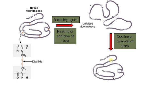
In this context, a very simple experiment 50 years ago, led some light on the protein folding mechanism. Cristian Anfisen was able to completely denature (unfold) the Ribonuclease A, by the addition of reducing agents and urea under heat treatment, and subsequently switch to normal conditions that allow the protein to re-fold fully functional. This experiment indicates that the amino acid sequence dictates the final structure. Notwithstanding some relevant exceptions, this has been largely confirmed.

Figure 3: The Anfinsen Dogma: Amino acid sequence dictated the final structure. From Anfinsen (1973) .

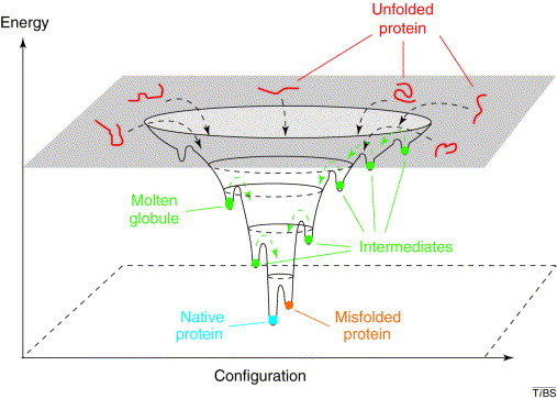
One can imagine that in vivo native structures of proteins look-alike the lowest free energy conformation, i.e., the global energy minimum. That is the basis of the funnel model of protein folding, which assumes that the number of possible conformations is reduced when a local energy minimum is achieved, constituting a path for the folding process.

Figure 4: Schematic diagram of a protein folding energy landscape according to the funnel model. Denatured molecules at the top of the funnel might fold to the native state by a myriad of different routes, some of which involve transient intermediates (local energy minima) whereas others involve significant kinetic traps (misfolded states). From .

Important

In conclusion, prediction of protein structures is possible, as protein folding relies only on the protein sequence, but it will require virtually infinite time and computational resources.

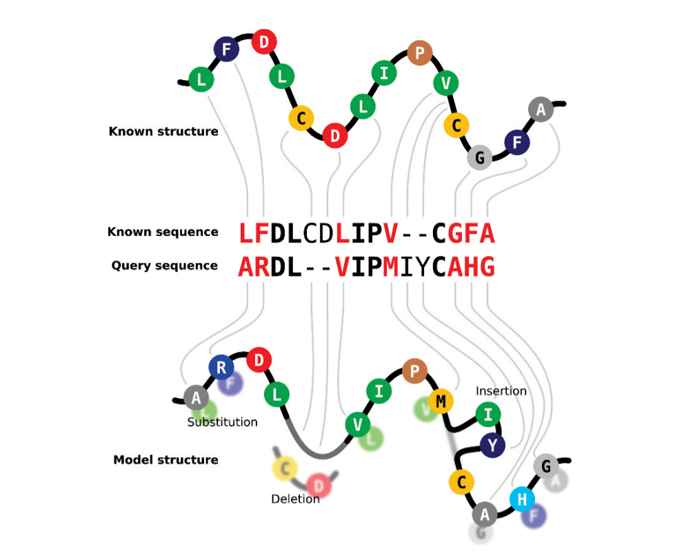
Homology modeling is one of the most convenient tricks to bypass that limitation. Basically, the strategy is adding all the possible extra information to the amino acid properties, namely the evolutionary conservation of sequences and structures.

Very often, before generating models you already have some information about your protein. For instance, if it is an enzyme you may have spotted the catalytic residues or substrate-interaction region. It is also advisable to check the literature, particularly if there is a companion paper of the related PDB structure(s) that may be available or that you can eventually find and use as the template(s) for modeling.

2 Homology modeling: Conservation is the key

Figure 5: Protein modeling in a nutshell is about going from the sequence to the structure. But, how do we do it?

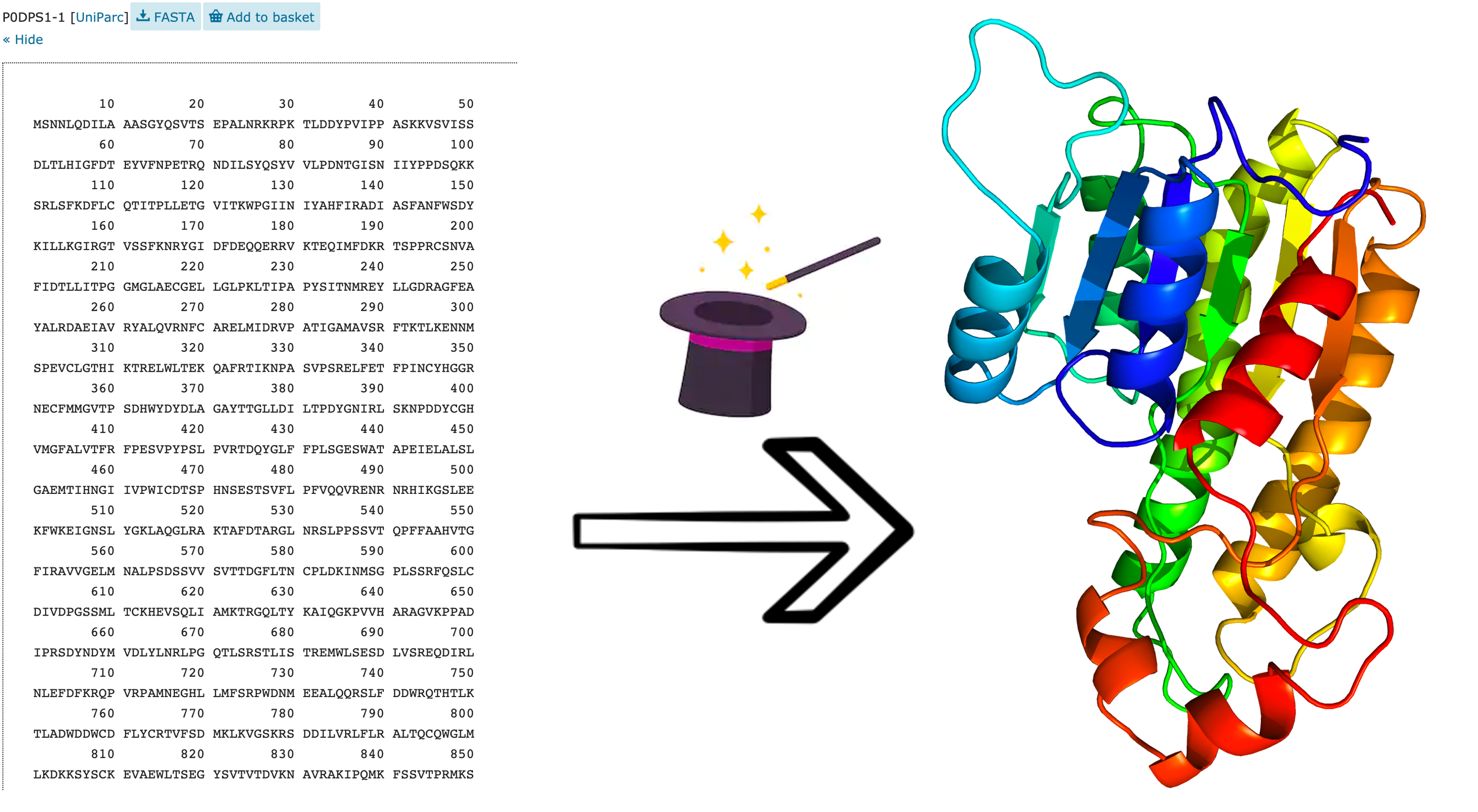
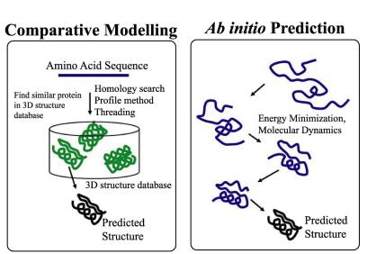
Traditionally and conceptually, the prediction of protein structures can be addressed from two different perspectives: comparative modeling and ab initio prediction. In the comparative modeling approach, one can predict 3D structure for protein sequences only if their homologs are found in the database of proteins with known structures. Obviously, the identification of such homologs is the keyword here. Until recently, most of the evolution in protein modeling was driven by the evolution of methods to identify distant sequence similarities that would reflex similar protein folds.

Figure 6: Two different approaches for structure prediction.

The accuracy of homology modeling will be limited by the availability of similar structures, ab initio predictions are limited by the mathematical models and computational resources, being often useful only with small peptides.

To maintain structure and function, certain amino acids in the protein sequence suffer a stronger selective pressure, evolving either slower than expected or within specific constraints, such as chemical similarity (i.e., conservative substitutions). Thus, homology modeling approaches assume that a similar protein sequence involves a similar 3D structure and function. At the same time, although the number of published sequences and structures continually increased, the number of unique folds remains almost steady since 2008.

Figure 7: Growth of the protein structure database since its inception in 1974. From Bonvin lab site.

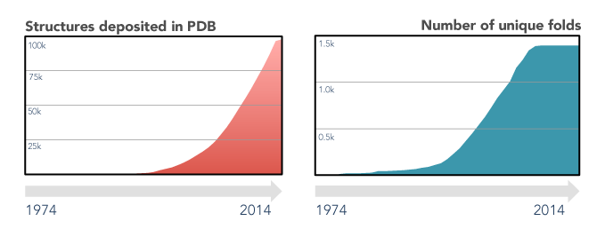
That implies that the space of protein sequences is much larger than the space of structures. This has been exploited by some structural databases, like Scop2 or CATH, that use hierarchical classifications of structures into very few categories of different structures.

Figure 8: CATH main categories exemplified the limited structures space, with 86k vs 500k domains in 2006 and 2022, respectively, but 40 and 41 architectures in the same years.

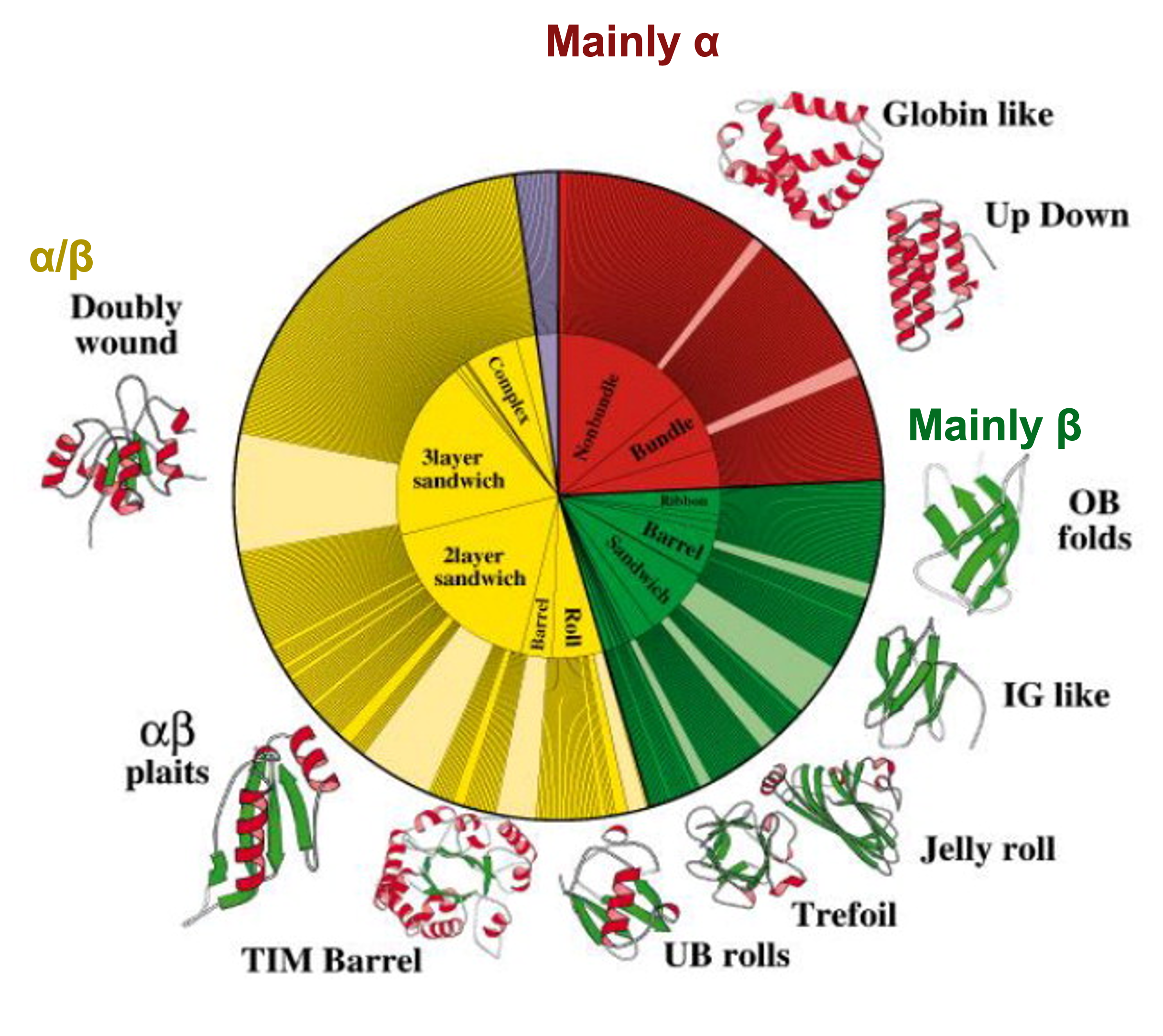
In conclusion, protein structures are more conserved than sequences, which allows for model construction by comparison of related proteins. Biological sequences evolve through mutation and selection and selective pressure is different for each residue position in a protein according to its structural and functional relevance. Sequence alignments attempt to tell us the evolutionary story of proteins.

3 Homology modeling in four steps

Figure 9: Workflow of template-based protein modeling. From Expasy Protein Structure, Comparative Protein Modelling, and Visualisation online course.

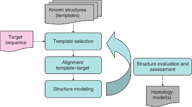
A basic workflow of homology modeling requires three steps: (1) identification of the best-suitable template, (2) alignment of the query sequence and the template, and (3) construction of the model. These steps can be addressed with diverse methodological alternatives and can provide different outputs that must be assessed (step 4) in order to decide the best solution for each step. For a more detailed review on homology modeling, I suggest reading Haddad, Adam, and Heger (2020).

In this course, we are focusing on end-to-end modeling with SWISS-MODEL (Waterhouse et al. 2018), a fully automated modeling server that allows you the construction of models without the requirement of a strong bioinformatics background or coding skills. The early versions of SWISS-MODEL only allowed modeling sequences with close homologs in databases but, as discussed below, implementation of advances in template recognition and model building, increased the modeling proficiency and accuracy, particularly during the last decade.

SWISS-MODEL has different supported inputs. Usually, you provide a single sequence query for template searching, but you can bypass this step and provide directly the template you want to use and even a template and a custom alignment. We will start with the first alternative.

3.0.0.1 In-class Homology Modeling exercise: Quick Modeling with SWISS-MODEL.

As an exercise, we are modeling a human DNA repair protein, NEIL2, and a viral DNA polymerase (HAdV-2 pol). We will intersperse discussion about modeling with the exercise steps.

Rather than provide just a recipe to make a model in two clics, the goal is to understand the process behind, while doing exercises with selected examples

3.1 Step 1+2. Template search and align.

3.1.1 Where can we search?

Template searching consists in finding a protein with known structure that has a sequence similar to our protein. As we mentioned above, the RCSB Protein Data Bank (PDB) is the largest database of protein structures, so we can search templates by comparing the sequence of our protein with the sequence of all the proteins in PDB. However, PDB was constructed to contain all the macromolecular structures, not for searching templates for modeling. Similar to other end-to-end software, SWISS-MODEL has its own curated database, called SMLT (SWISS-MODEL template library). This is based on PDB, updated weekly, and also annotated and indexed to boost searches. As of 6 July 2022, SMLT contains 133,049 unique protein sequences that map to 332,864 biological units.

Now, you first need your sequences. A protein sequence database like Uniprot or NCBI Protein, is a good place for this task.

If you want to cheat yourself, I give you the HAdV-2pol and NEIL2 sequences.

3.1.2 How can we search accurately and fast?

Figure 10: Query-template alignment is the base for homology modeling (Kelley 2009)

Finding templates require comparing sequences, thus an accurate and powerful alignment method is essential. Comparing one protein sequence with a whole database is time-consuming, as you will compare with totally unrelated proteins, which is a loss of resources. Two basic improvements increased the template search capacity, (1) the introduction of secondary structure (SS) by comparing SS predictions of the query protein and the secondary structures of the protein database, and (2) the use of profiles to make easier the comparison. Profiles are a mathematical way to summarize a multiple sequence alignment in which the frequency of each amino acid at each position is quantified. A particular type of profiles, the Hidden Markov Models (HMM) are very well suited to search databases for similar sequences. HMMs include amino acid insertions and deletions, meaning that they can model entire alignments, including divergent regions. This allows the identification of highly conserved positions that not only define the protein function but also the fold. For instance, glycine residues at the end of each beta-strand or a pattern of polar residues that favors alpha-helices. A previous comparison of the query sequence with a database of sequences will allow us to include evolutionary information about it. Therefore, we moved from a requirement of >30% identity to obtain good models before the implementation of profiles, to good models even with ⁓20% identity or below. Moreover, the generation of profiles also facilitates clustering of the search database, reducing search time. The implementation of these capacities led to the implementation of the so-called fold recognition in homology modeling.

Figure 11: From sequence vs. sequence search to profile-profile comparison (Kelley 2009).

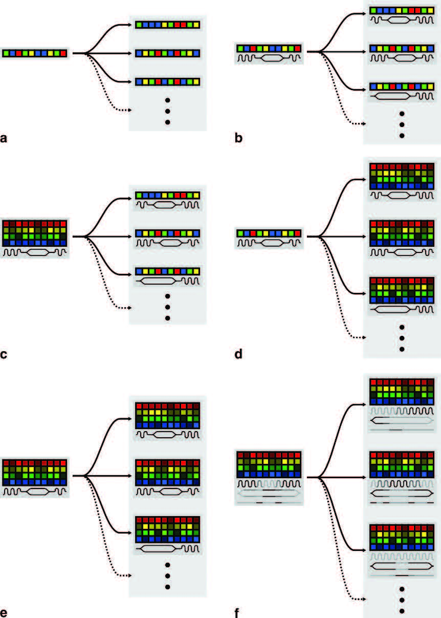
Template searches in SWISS-MODEL have evolved through the years and currently, this step is performed with HHblits (Remmert et al. 2011), a specific profile-profile method. We could search for templates also with Blast or other profile-profile methods, like Psi-BLAST, HHPred, or JackHMMER. Then, templates are ranked by two different numeric parameters ranging between 0 and 1: GMQE (global model quality estimate) and QSQE (quaternary structure quality estimate). Briefly, GMQE uses probability functions to assess several properties of the target-template alignment (sequence identity, sequence similarity, HHblits score, the agreement between predicted secondary structure of target and template, the agreement between predicted solvent accessibility between target and template; all normalized by alignment length) to predict the expected quality of the resulting model. QSQE assesses the oligomeric state probability of the model.

Note: If you click on “Build Model”, it will directly use the top-ranked template, so you’ll miss some fun, but you can go back for that later on if you change your mind.

Figure 12: SWISS-MODEL modeling start. Just paste your sequences and click on Search.

3.1.2.1 Could you foresee which of our queries will give rise to a better model? Why?

3.2 Step 3. Model Building.

By default, SWISS-MODEL will provide 50 ranked possible templates. The output also contains information about the method and resolution of the templates, the % of identity (and alignment coverage) with the query sequence, and the GMQE and QSQE.

The top template is marked by default and it likely will give the best model, but it is also interesting to try some alternative templates depending on the downstream application of the model (see below). For instance with a different substrate/cofactor that can have a key role in the protein function or with different coverage or % identity.

Once the template(s) is selected, model coordinates are constructed based on the alignment of the query and template sequence using ProMod3 module (Studer et al. 2021). SWISS-MODEL uses a fragment assembly, which is also the bases of Fold-recognition or Threading methods (see Threading section). Other programs, like Modeller, are based in the satisfaction of general spatial restraints (Giacomo Janson et al. 2019). Modeller is a command-line tool that allow full customization of the modeling, which requires more knowledge about the process but can be very useful for some types of proteins. However, it has been implemented in some online servers (ModWeb) and user-friendly applications, including ChimeraX and Pymol (Pymod plugin, G. Janson and Paiardini (2021)). Modeller can be also called from the HHPred output (if you included PDB as a searchable database), which is very convenient to model remote homologs using several templates in a few minutes.

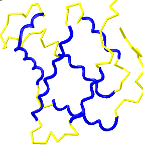
Fragment assembly will use the template core backbone atoms to build a core structure of the model, leaving non-conserved regions (mostly loops) for later. Loops modeling includes the use of a homologs subset of a dedicated loop database, Monte Carlo sampling as a fallback and even ab initio building or missing loops.

Figure 13: Backbone and loop modeling. From Expasy Protein Structure, Comparative Protein Modelling, and Visualisation.

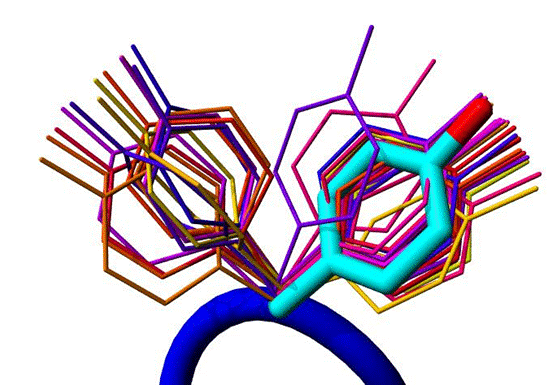
Then, positioning of side chain of non conserved amino acids is undertook. The goal is finding the most likely side chain conformation, using template structure information, rotamer libraries (from a curated set known protein structures) and energetic and packaging criteria. If many side chains have to be placed in the structure it will lead to a “chicken and egg problem”, as positioning one rotamer would affect others. That means that identification of possible hydrogen bonds between residues side chains and between side chains and the backbone reduce the optimization calculations. At the end of the day, the more residues correctly positioned, the best model.

Figure 14: Side chain modeling. From CMBI Seminars on Bioinformatics.

Finally, a short energy minimization is carried out to reduce the unfavorable contacts and bonds by adapting the angle geometries and relax close contacts. This energy minimization step or refinement can be useful to achieve better models but only when the folding is already accurate.

3.3 Step 4. Result assessing.

The computer always give you a model but it doesn’t mean that you have a model that makes sense. How can we know if we can rely on the model? Output models are colored in a temperature color scale, from navy blue (good quality) to red (bad quality). That can help us to understand our model in a first sight. Also, this is an interactive site and you can zoom-in, zoom-out the model. Many other features are available to work on your model. For instance, you can compare multiple models, you can change the display options. You can also download all the files and reports on the “Project Data” button.

Figure 15: NEIL2 model created with SWISS-MODEL (July 2022)

There is also a “Structure Assessment” option. This provide you a detailed report of the structural problems of your model. You can see Ramachandran plots that highlight in red the amino acid residues with abnormal phi/psi angles in the model and a detailed list of other problems.

The GMQE is updated to the QMEAN Zscore and QMEANDisCo (Studer et al. 2020). The QMEAN Z-score or the normalized QMEAN score indicates how the model is comparable to experimental structures of similar size. A QMEAN Z-score around 0 indicates good agreement, while score below -4.0 are given to models of low quality. Besides the number, a plot shows the QMEAN score of our model (red star) within all QMEAN scores of experimentally determined structures compared to their size. Overall, the Z-score is equivalent to the standard deviation of the mean.

Figure 16: Per-residue QMEANDisCo scores are mapped as red-to-green colour gradient on a model of lbp-8 in Caenorhabditis elegans (UniProtKB: O02324, PDB: 6C1Z). Distance constraints have been constructed from an ensemble of experimentally determined protein structures that are homologous to lbp-8. The inset depicts two example constraints between residues marked with colour-coded spheres in the model. From Studer et al. (2020).

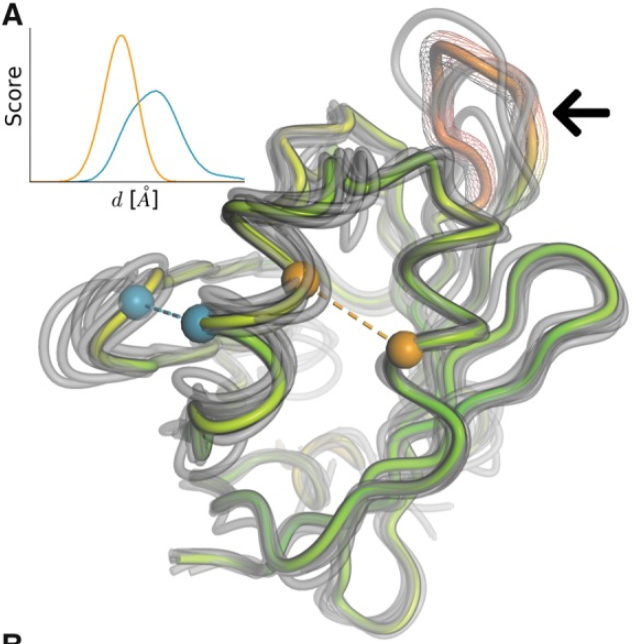
The QMEANDisCO was implemented in SWISS-MODEL in 2020 and it is a powerful, single parameter that combines statistical potentials and agreement terms with a distance constraints (DisCo) to provide a consensus score. DisCo evaluates consistencies of pairwise CA-CA distances from a model with constraints extracted from homologous structures. All scores are combined using a neural network trained to predict per-residue scores. We can check a global score, but also a local score for each residue, that help us to understand which regions of the model are more likely to accurately folded (i.e. they are more reliable).

Figure 17: HAdV-2 DNA polymerase model obtained with SWISS-MODEL (July 2022).

QMEANDisCo can be used to analyze models obtained with other methods in order to make them comparable (note that you can use QMEANDisCo for models obtained with any method, you just need a .pdb file). There are other independent model assessing tools commonly used to assess protein models, like VoroMQA [Olechnovič and Venclovas (2017)] or MoldFold (McGuffin et al. 2021). VoroMQA is very quick method that combines the idea of statistical potentials (i.e. a knowledge-based score function) with the use of interatomic contact areas to provide a score in the range of [0,1]. When applied to PDB database, most of the high-quality experimentally-based structures have a VoroMQA score >0.4. Thus, if the score is greater than 0.4, then the model is likely good and models with score <0.3 are likely bad ones. Models with score 0.3-0.4 are uncertain and should not be classified with VoroMQA. On the other hand, ModFold is a meta-tool that provides you a very detailed report (and parseable files) with local and global scores, but it can take hours/days to obtain the result, so tend to use it only with selected models.

Another key parameter that you should know if you want to compare protein structures is the alpha carbon RMSD (see Structure alignment section). Any protein structural alignment will give you this parameter as an estimation of the difference of the structures. You can align structure with many online servers, like RCSB, FATCAT2 or using molecular visualization apps, like ChimeraX or PyMOL (see Protein Structure Display section).

3.3.0.1 Which model is better? Which regions are more difficult to model? Why?

3.4 Corollary: What can I do with my model and what I cannot?

Figure 18: Accuracy and application of protein structure models (in 2001). From .

A big power entails a big responsibility. The use of models entails a precaution and a need for experimental validation. However, knowing the limitations of our model is required for a realist use of it; and limits are defined by the model quality.

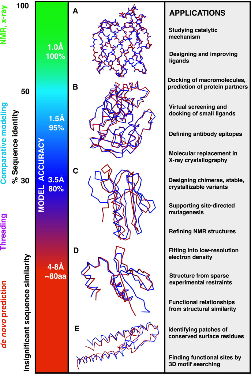
The accuracy of a comparative model is related to the percentage sequence identity on which it is based. High-accuracy comparative models can have about 1-2 Å root mean square (RMS) error for the main-chain atoms, which is comparable to the accuracy of a nuclear magnetic resonance (NMR) structure or an x-ray structure. These models can be used for functional studies and the prediction of protein partners, including drugs or other proteins working in the same process. Also, for some detailed studies, it would be convenient to refine your model by Molecular Dynamics and related methods towards a native-like structure. I suggest checking the review by Adiyaman and McGuffin (2019) on this topic.

On the contrary, low-accuracy comparative models are based on less than 20-30% sequence identity, hindering the modeling capacity and accuracy. Some of these models can be used for protein engineering purposes or to predict the function of orphan sequences based on the protein fold (using Dali or Foldseek).

As mentioned above, it also advisable to check the template structures and read the papers describing them in order to squeeze all the information from your model.

What do you think you could use our models of NEIL2 and HAdV-2pol?

4 Homology Modeling Practice

This is a Evernote note that you can consult online and also copy into your Evenote account if you wish.

References

Adiyaman, Recep, and Liam James McGuffin. 2019. “Methods for the Refinement of Protein Structure 3D Models.” International Journal of Molecular Sciences 20 (9): E2301. https://doi.org/10.3390/ijms20092301.

Anfinsen, C. B. 1973. “Principles that govern the folding of protein chains.” Science (New York, N.Y.) 181 (4096): 223–30. https://doi.org/10.1126/science.181.4096.223.

Haddad, Yazan, Vojtech Adam, and Zbynek Heger. 2020. “Ten Quick Tips for Homology Modeling of High-Resolution Protein 3d Structures.” PLOS Computational Biology 16 (4): e1007449. https://doi.org/10.1371/journal.pcbi.1007449.

Janson, Giacomo, Alessandro Grottesi, Marco Pietrosanto, Gabriele Ausiello, Giulia Guarguaglini, and Alessandro Paiardini. 2019. “Revisiting the “Satisfaction of Spatial Restraints” Approach of MODELLER for Protein Homology Modeling.” PLOS Computational Biology 15 (12): e1007219. https://doi.org/10.1371/journal.pcbi.1007219.

Janson, G., and A. Paiardini. 2021. “PyMod 3: a complete suite for structural bioinformatics in PyMOL.” Bioinformatics 37 (May): 1471–72. https://doi.org/10.1093/bioinformatics/btaa849.

Kelley, Lawrence A. 2009. “Fold Recognition.” In, edited by Daniel John Rigden, 27–55. Dordrecht: Springer Netherlands. https://doi.org/10.1007/978-1-4020-9058-5_2.

Kendrew, J. C., G. Bodo, H. M. Dintzis, R. G. Parrish, H. Wyckoff, and D. C. Phillips. 1958. “A three-dimensional model of the myoglobin molecule obtained by x-ray analysis.” Nature 181 (4610): 662–66. https://doi.org/10.1038/181662a0.

Manjasetty, Babu A., Andrew P. Turnbull, Santosh Panjikar, Konrad Büssow, and Mark R. Chance. 2008. “Automated Technologies and Novel Techniques to Accelerate Protein Crystallography for Structural Genomics.” PROTEOMICS 8 (4): 612–25. https://doi.org/10.1002/pmic.200700687.

McGuffin, Liam J., Fahd M. F. Aldowsari, Shuaa M. A. Alharbi, and Recep Adiyaman. 2021. “ModFOLD8: accurate global and local quality estimates for 3D protein models.” Nucleic Acids Research 49 (W1): W425–30. https://doi.org/10.1093/nar/gkab321.

Muhammed, Muhammed Tilahun, and Esin Aki-Yalcin. 2019. “Homology modeling in drug discovery: Overview, current applications, and future perspectives.” Chemical Biology & Drug Design 93 (1): 12–20. https://doi.org/10.1111/cbdd.13388.

Olechnovič, Kliment, and Česlovas Venclovas. 2017. “VoroMQA: Assessment of protein structure quality using interatomic contact areas.” Proteins 85 (6): 1131–45. https://doi.org/10.1002/prot.25278.

Remmert, Michael, Andreas Biegert, Andreas Hauser, and Johannes Söding. 2011. “HHblits: lightning-fast iterative protein sequence searching by HMM-HMM alignment.” Nature Methods 9 (2): 173–75. https://doi.org/10.1038/nmeth.1818.

Studer, Gabriel, Christine Rempfer, Andrew M. Waterhouse, Rafal Gumienny, Juergen Haas, and Torsten Schwede. 2020. “QMEANDisCo-distance constraints applied on model quality estimation.” Bioinformatics (Oxford, England) 36 (6): 1765–71. https://doi.org/10.1093/bioinformatics/btz828.

Studer, Gabriel, Gerardo Tauriello, Stefan Bienert, Marco Biasini, Niklaus Johner, and Torsten Schwede. 2021. “ProMod3-A versatile homology modelling toolbox.” PLoS computational biology 17 (1): e1008667. https://doi.org/10.1371/journal.pcbi.1008667.

Waterhouse, Andrew, Martino Bertoni, Stefan Bienert, Gabriel Studer, Gerardo Tauriello, Rafal Gumienny, Florian T Heer, et al. 2018. “SWISS-MODEL: Homology Modelling of Protein Structures and Complexes.” Nucleic Acids Research 46 (W1): W296–303. https://doi.org/10.1093/nar/gky427.